Use this facility to create histograms of measured data from Monte Carlo Simulation results. This feature is the same as using the Performance Analysis Random Probe tool.
Shortcuts
Default Keys: None
Default Menu: Simulation
Command: Plot Histogram
How To Plot A Monte Carlo Histogram
First run a Monte Carlo Simulation. Make sure you use a reasonable number of runs, 25 at an absolute minimum and preferably 100 or more.
Next use the Plot Histogram option from the Monte Carlo sub-menu on the Simulation menu.
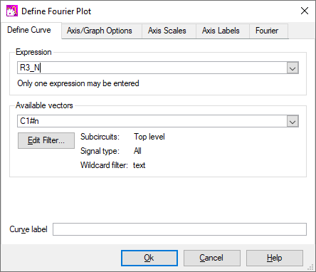
The Define Performance Analysis dialog will be displayed:-

When running multi-step analyses which generate multiple curves, it is often useful to be able to plot some characteristic of each curve against the stepped value. A range of functions, sometimes known as “goal functions”, are available that perform a computation on a complete curve to create a single value. By applying one or a combination of these functions on the results of a multi- step analysis, a curve of the goal function versus the stepped variable may be created.
In the Expression field, enter the goal function and the signal you wish to apply the function to. Use the Functions button to view the available functions from the simulator help pages. Use the Available Vectors list to select the signal of interest.
For more information on how to use the Performance Analysis dialog, use the Pulsonix-Spice Simulator’s help topics.
Press OK and the histogram will be calculated and a progress box will be displayed while this is happening. This can take a considerable time especially for a large number of runs. If it is taking too long, press Ctrl+Q to abort the operation. You will still see the result that has been obtained up to the time that the process was stopped.
Multi-Step Monte Carlo Example
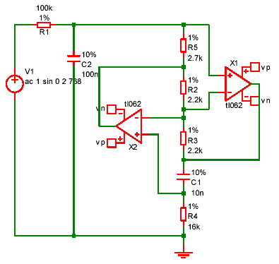
This is a design for an active band pass filter using the simulated inductor method. See “Examples\Spice\MonteCarlo\768Hz_bandpass”. We want to plot a histogram of the centre frequency of the filter.

The example circuit has been set up to do 100 runs. This will not take long to run, less than 10 seconds on most machines. This is the procedure:
-
Run the simulation using F9 or Simulate Design option.
-
Select Plot Histogram option.
-
Enter net N0000 in the expression box. This is the output of the filter, at the junction of R1 and C2. We must now modify this with a goal function that returns the centre frequency. The function CentreFreq will do this. This measures the centre frequency by calculating the half way point between the intersections at some specified value below the peak. Typically you would use 3dB.
Modify the value in the expression box so that it reads:
CentreFreq(N0000, 3)
-
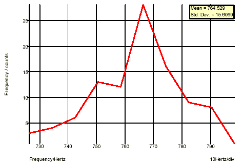
At this stage you can optionally modify the graph setting to enter your own axis labels etc. Now press OK. This is what you should see:

Note that the mean and standard deviation are automatically calculated.
Histograms for Single Step Monte Carlo Sweeps
An example of this type of run is “Examples\Spice\Sweep\AC_Param_Monte”. These runs produce only a single curve with each point in the curve the result of the Monte Carlo analysis. With these runs you do not need to apply a goal function, just enter the name of the signal you wish to analyse.
- Open the example circuit “Examples\Spice\Sweep\AC_Param_Monte”.
- Run simulation.
- Select Plot Histogram.
- Type “Vpos-VNeg” in the expression box. “VPos” is the net on the ’+’ pin of the differential amplifier E1, and “VNeg” is the net on the ’-’ pin of E1.
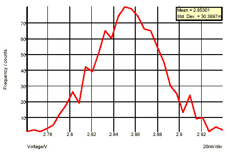
- Press OK. You should see something like this:

This is a histogram showing the distribution of the gain of the amplifier at 100kHz.
Related Topics
Define Component Value | Define Spice Type | Matching Components | Monte Carlo Simulation | Monte Carlo Tolerances | Random Probe | Set Device Tolerance | Set Match Tolerance